Introduction to Vector Databases

What's in this lesson: Vector embeddings, similarity search, indexing techniques (HNSW, IVF, PQ), ANN search, metadata filtering, RAG applications, and scaling strategies.
Why this matters: Vector databases power modern AI applications like semantic search, recommendation systems, and retrieval-augmented generation (RAG), enabling machines to understand and find similar content in ways traditional databases cannot.

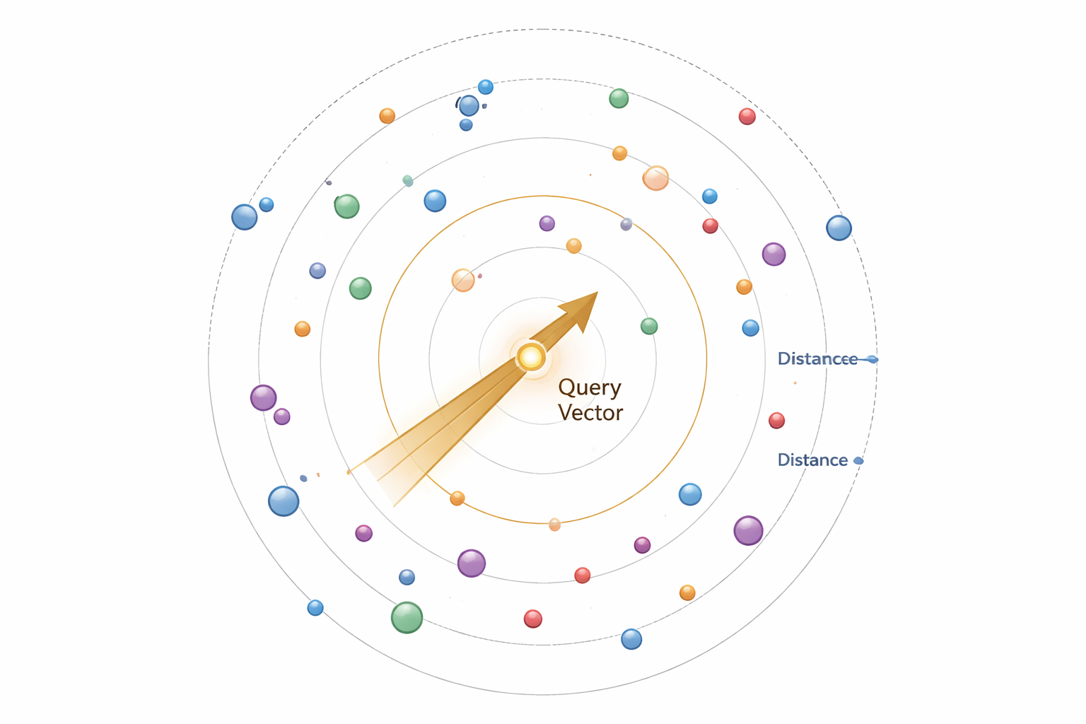
🎯 Attention Activity: Find Similar Points

Click anywhere in the space below to place a query point. Watch as the system highlights similar vectors based on distance!

What you just experienced: This is the core concept of vector databases—finding similar items in high-dimensional space. Each point represents data (like a document, image, or product), and proximity indicates similarity.

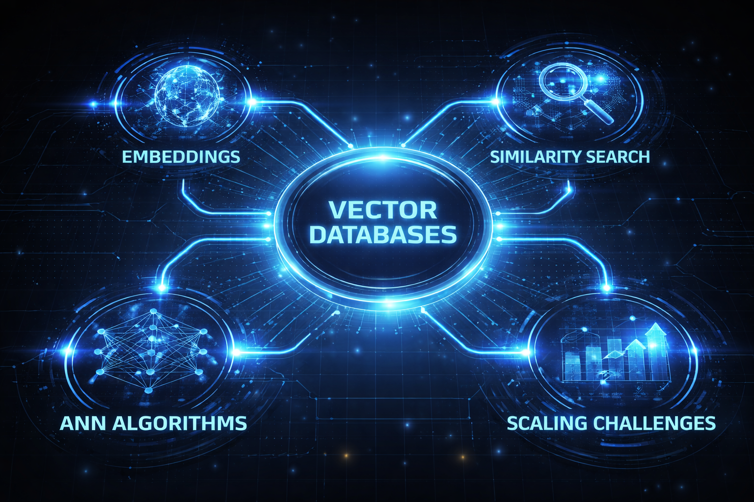
What Are Vector Databases?

Vector databases are specialized systems designed to store, index, and query high-dimensional vector embeddings efficiently. Unlike traditional databases that store structured data in rows and columns, vector databases handle numerical representations of unstructured data.

Key Characteristics

High-dimensional storage: Handle vectors with hundreds or thousands of dimensions
Similarity search: Find nearest neighbors rather than exact matches
Specialized indexing: Use algorithms optimized for vector operations
Scalability: Manage billions of vectors with sub-millisecond latency

Traditional vs. Vector Databases

Traditional: "Find users WHERE age > 25 AND city = 'NYC'"
Vector: "Find documents most similar to this query embedding"

Embeddings and Vector Representation

Embeddings are dense numerical representations that capture semantic meaning. Machine learning models transform unstructured data (text, images, audio) into fixed-size vectors where similar items are close together in vector space.

How Embeddings Work

Transformation: Neural networks encode input data into vectors
Dimensionality: Typical sizes: 384, 768, 1536, or 4096 dimensions
Semantic capture: Similar meanings → similar vectors
Distance preservation: Geometric distance reflects conceptual similarity

Example: Text Embeddings

"The cat sat on the mat" → [0.23, -0.45, 0.67, ..., 0.12]
"A feline rested on the rug" → [0.21, -0.43, 0.65, ..., 0.15]

These sentences have different words but similar embeddings because they convey the same meaning.

Popular Embedding Models

OpenAI Ada-002: 1536 dimensions, general-purpose
BERT: 768 dimensions, contextual understanding
Sentence-BERT: Optimized for sentence similarity
CLIP: Multi-modal (text + images)

Similarity Search and Distance Metrics

Similarity search finds vectors closest to a query vector. The definition of "closest" depends on the distance metric you choose.

Common Distance Metrics

Click each metric to see its characteristics:

Euclidean (L2)

Straight-line distance. Best for spatial data.

d = √Σ(a-b)²

Cosine Similarity

Measures angle, ignores magnitude. Best for text.

sim = a·b / (||a|| ||b||)

Dot Product

Magnitude-aware similarity. Fast computation.

d = Σ(aᵢ × bᵢ)

Manhattan (L1)

Grid-based distance. Robust to outliers.

d = Σ|a-b|

Choosing the Right Metric

Text/Semantic search: Cosine similarity (direction matters, not magnitude)
Image embeddings: Euclidean distance (spatial relationships)
High-dimensional sparse data: Dot product (computational efficiency)
Outlier-sensitive tasks: Manhattan distance (more robust)

Knowledge Check 1

Which distance metric is most commonly used for text embeddings and why?

Euclidean distance, because it measures exact magnitude differences Cosine similarity, because it focuses on direction rather than magnitude Manhattan distance, because text data is grid-structured Dot product, because it's the fastest to compute

Indexing Techniques: HNSW, IVF, PQ

Brute-force search (comparing against every vector) becomes impractical with millions or billions of vectors. Indexing structures enable fast approximate searches.

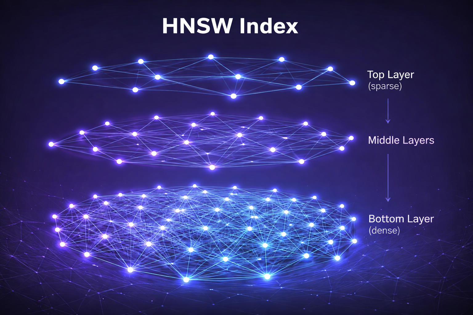
1. HNSW (Hierarchical Navigable Small World)

Graph-based index with multiple layers. Top layers are sparse for fast routing, bottom layers are dense for precision.

Strengths: Excellent recall, fast queries, good for high-dimensional data
Weaknesses: High memory usage, slow indexing time
Best for: When query accuracy is critical and memory isn't constrained

HNSW Layer Visualization (hover over nodes):

Layer 2:

1

5

(Entry points)

Layer 1:

1

3

5

7

9

(Routing layer)

Layer 0:

1

2

3

4

5

6

7

8

9

10

(All vectors)

2. IVF (Inverted File Index)

Clustering-based index that partitions vectors into clusters (Voronoi cells), then searches only relevant clusters.

Strengths: Memory efficient, fast indexing, good for 1M-100M vectors
Weaknesses: Lower recall than HNSW, requires careful tuning
Best for: Large-scale systems with memory constraints

3. PQ (Product Quantization)

Compression technique that splits vectors into subvectors and quantizes each independently, drastically reducing memory.

Strengths: 10-50x memory reduction, enables billion-scale search
Weaknesses: Lossy compression reduces accuracy
Best for: Combined with IVF (IVF-PQ) for massive datasets

Approximate Nearest Neighbor (ANN) Search

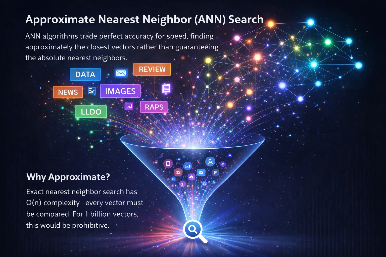
ANN algorithms trade perfect accuracy for speed, finding approximately the closest vectors rather than guaranteeing the absolute nearest neighbors.

Why Approximate?

Exact nearest neighbor search has O(n) complexity—every vector must be compared. For 1 billion vectors with 1536 dimensions, a single query could take seconds. ANN reduces this to milliseconds with 95-99% recall.

The Accuracy-Speed Trade-off

Brute Force (100% recall) ~1000ms

IVF-PQ (98% recall) ~50ms

HNSW (99% recall) ~5ms

Key ANN Algorithms

HNSW: Graph-based, best recall/speed balance
FAISS (IVF-PQ): Facebook's library, scales to billions
ANNOY: Tree-based, memory-efficient
ScaNN: Google's algorithm, optimized for large batches

Tuning Parameters

Recall target: Higher recall = slower queries but better results
Index size: More memory = faster queries
Build time: Complex indexes take longer to construct

Knowledge Check 2

What is the primary advantage of HNSW over IVF-based indexing methods?

HNSW uses less memory than IVF indexes HNSW provides higher recall and faster query times, especially for high-dimensional data HNSW can index vectors faster than IVF methods HNSW works better with compressed vectors

Metadata Filtering and Hybrid Search

Real-world applications often need more than just semantic similarity—they combine vector search with traditional filters and full-text search.

Metadata Filtering

Attach structured metadata to vectors and filter before or during search:

Pre-filtering: Filter candidates first, then search vectors (can reduce search space but may miss results)
Post-filtering: Search vectors first, then filter results (maintains recall but less efficient)
Inline filtering: Filter during search traversal (best balance, requires index support)

Example Query:

Find documents similar to "machine learning optimization"
WHERE author = "Smith" AND year >= 2022
AND category IN ["AI", "ML"]

Hybrid Search

Combines multiple search methods for better results:

Vector + Keyword: Semantic understanding + exact term matching
Dense + Sparse: Neural embeddings + BM25 or TF-IDF
Multi-modal: Text + image vectors simultaneously

Fusion Strategies

Reciprocal Rank Fusion (RRF): Combines rankings from multiple sources
Weighted scoring: Assign weights to vector vs. keyword results
Reranking: Use vector search for recall, then rerank with more expensive models

Popular Vector Databases with Hybrid Search

Qdrant: Advanced filtering, payload indexing
Weaviate: Hybrid search with BM25 + vector
Pinecone: Metadata filtering, sparse-dense vectors
Milvus: Scalar filtering, hybrid search support

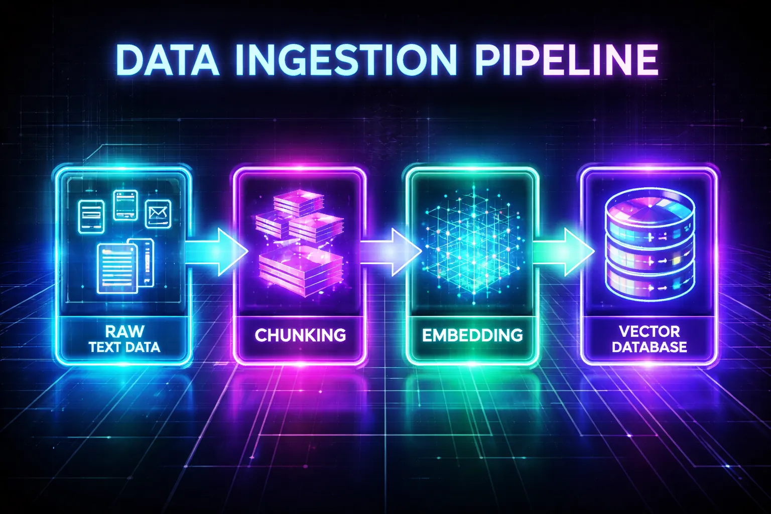
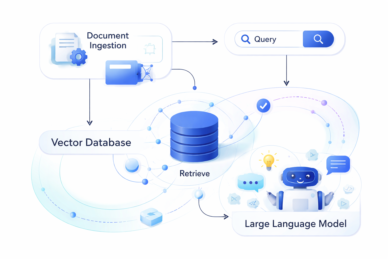
Data Ingestion and Query Pipelines

Building production vector search requires well-designed pipelines for both ingestion (adding data) and querying (retrieving data).

Ingestion Pipeline

Click the button to see the pipeline in action:

📄

Raw Data

Text, images, audio

✂️

Chunking

Split into segments

🧠

Embedding

Generate vectors

🗂️

Metadata

Attach attributes

💾

Index & Store

Build index structure

Query Pipeline

User query: Natural language input
Query embedding: Convert to vector using same model
Retrieval: ANN search with filters
Reranking (optional): Refine results with cross-encoders
Post-processing: Format and return results

Best Practices

Chunk size: 200-500 tokens for text balances context and precision
Overlap: 10-20% overlap between chunks prevents information loss
Same embedding model: Use identical model for indexing and querying
Batch processing: Embed and index in batches for efficiency
Version tracking: Track embedding model versions for reproducibility

Knowledge Check 3

In a hybrid search system, what is the main advantage of using Reciprocal Rank Fusion (RRF)?

It reduces the computational cost of vector similarity calculations It effectively combines rankings from multiple search methods without requiring score normalization It compresses vectors to save storage space It automatically selects the best distance metric for each query

Scaling, Sharding, and Performance Optimization

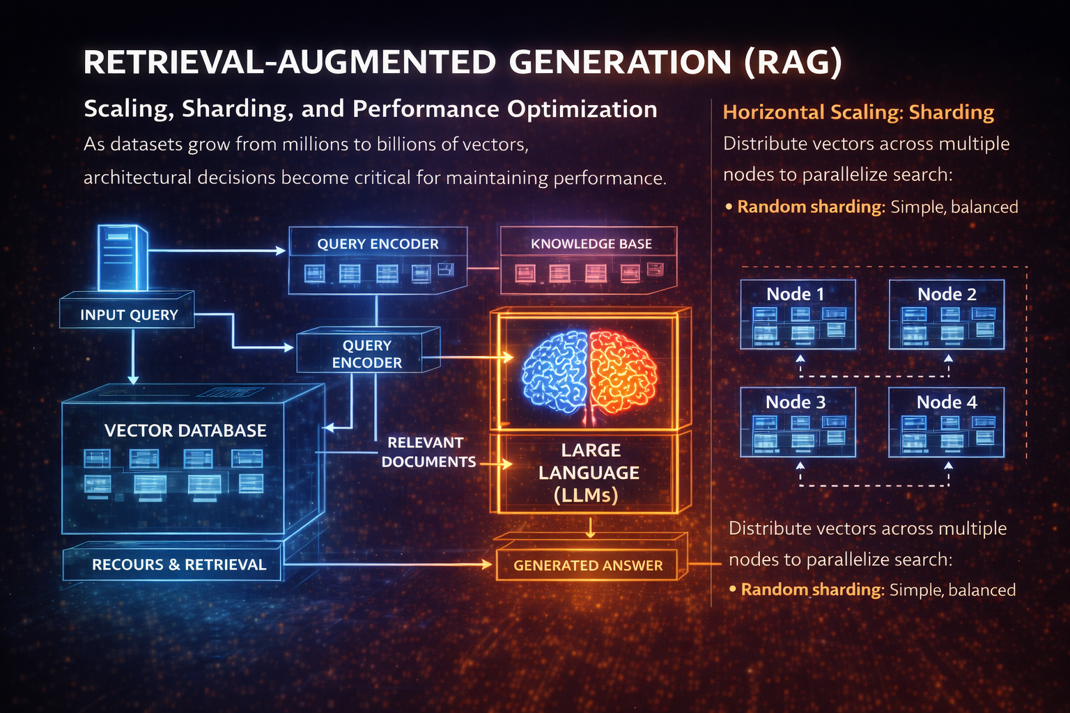
As datasets grow from millions to billions of vectors, architectural decisions become critical for maintaining performance.

Horizontal Scaling: Sharding

Distribute vectors across multiple nodes to parallelize search:

Random sharding: Simple, balanced distribution
Hash-based sharding: Consistent placement by metadata
Cluster-based sharding: Group similar vectors (locality-sensitive)

Example: 100M vectors across 10 shards

• Each shard: 10M vectors → faster local search
• Query all shards in parallel → aggregate results
• Total latency ≈ single shard latency + network overhead

Vertical Scaling: Resource Optimization

Memory: Keep hot indexes in RAM, cold data on SSD
CPU: Use SIMD instructions for vector operations
GPU: Batch queries for massive parallelism
Compression: PQ reduces memory by 10-50x

Caching Strategies

Query caching: Store results for repeated queries
Embedding caching: Cache frequently accessed vectors
Negative caching: Remember what's NOT similar

Performance Benchmarks (typical)

10M vectors:
1-5ms p95 latency

100M vectors:
5-20ms p95 latency

1B vectors:
20-50ms p95 latency

10B+ vectors:
50-200ms p95 latency

Cost Optimization

Dimensionality reduction: PCA/UMAP to reduce vector size
Quantization: Trade precision for storage (float32 → int8)
Tiered storage: Recent data in-memory, archive on disk
Batch updates: Rebuild indexes periodically vs. real-time

Use Cases: Retrieval-Augmented Generation (RAG)

RAG has become one of the most important applications of vector databases, powering AI assistants with current, domain-specific knowledge.

How RAG Works

Index knowledge base: Embed documents into vector database
User query: Convert question to embedding
Retrieve context: Find most relevant document chunks
Augment prompt: Inject retrieved context into LLM prompt
Generate response: LLM produces grounded, factual answer

Why RAG + Vector Databases?

Up-to-date information: Update knowledge base without retraining LLM
Domain expertise: Add proprietary or specialized knowledge
Reduced hallucination: Ground responses in retrieved facts
Source attribution: Cite specific documents or sections
Cost efficiency: Cheaper than fine-tuning large models

RAG Challenges

Context window limits: LLMs can only process finite tokens
Retrieval quality: Poor retrieval = poor generation
Chunk boundaries: Important info might span chunks
Latency: Retrieval adds 20-100ms to response time

Advanced RAG Techniques

Hypothetical document embeddings (HyDE): Generate fake answer, use it for retrieval
Reranking: Use cross-encoder to refine top-k results
Multi-query: Generate multiple query variations for better coverage
Iterative retrieval: Retrieve, reason, retrieve again based on initial findings

More Use Cases and Applications

Beyond RAG, vector databases enable a wide range of AI-powered applications across industries.

🔍 Semantic Search

E-commerce: "Show me comfortable running shoes for winter" (not just keyword match)
Enterprise search: Find documents by meaning, not exact words
Code search: Find similar code patterns or functionality

🎯 Recommendation Systems

Content recommendations: Netflix, YouTube, Spotify
Product recommendations: Amazon, eBay
Social feeds: LinkedIn, Twitter/X personalization
Collaborative filtering: "Users similar to you liked..."

🖼️ Multi-modal Search

Image search: Find images by text description or similar image
Video search: Search within video content semantically
Audio search: Find similar music or speech patterns
Cross-modal: Text query → image results (CLIP embeddings)

🛡️ Anomaly Detection

Fraud detection: Identify unusual transaction patterns
Cybersecurity: Detect abnormal network behavior
Quality control: Find defective products in manufacturing

🤖 AI Agents & Memory

Long-term memory: Store conversation history, retrieve relevant context
Semantic memory: Remember facts and relationships
Episodic memory: Recall past interactions and events

🧬 Scientific Research

Drug discovery: Find similar molecular structures
Genomics: Compare DNA/protein sequences
Literature review: Discover related research papers

Real-world Examples

Notion AI: Semantic search across user documents
Shopify: Product recommendations and search
GitHub Copilot: Code similarity and suggestions
Duolingo: Personalized learning recommendations

Knowledge Check 4

What is the primary benefit of using vector databases in RAG systems compared to traditional keyword-based retrieval?

Vector databases are always faster than keyword search engines Vector databases retrieve semantically relevant content even when exact keywords don't match Vector databases require less storage space than traditional databases Vector databases eliminate the need for document chunking

Challenges and Future Trends

Vector database technology is rapidly evolving. Understanding current limitations and future directions is essential for building robust systems.

Current Challenges

Cost at scale: Storing billions of high-dimensional vectors is expensive
Cold start problem: New items lack sufficient data for good embeddings
Embedding drift: Model updates change vector spaces, requiring reindexing
Interpretability: Hard to explain why specific results were retrieved
Multi-tenancy: Isolating data for different customers efficiently
Real-time updates: Balancing index freshness with query performance

Emerging Solutions

Binary quantization: Extreme compression with minimal accuracy loss
Matryoshka embeddings: Variable-dimension vectors for flexibility
Streaming indexes: Real-time updates without full rebuilds
Serverless vector databases: Pay-per-query, auto-scaling

Future Trends (2024-2026)

Native LLM integration: Vector DBs with built-in reasoning
Multi-modal by default: Text, image, audio in unified space
Federated vector search: Search across distributed, private databases
Hardware acceleration: Custom chips (DPUs, AI accelerators) for vector ops
Graph + vector fusion: Combining knowledge graphs with embeddings
Adaptive indexes: Self-tuning based on query patterns

Research Directions

Learned indexes: ML models that predict vector locations
Quantum-inspired algorithms: Novel approaches to high-dimensional search
Privacy-preserving search: Encrypted vector search (homomorphic encryption)
Dynamic embeddings: Context-aware vectors that change with time or user

Industry Landscape

Major players: Pinecone, Weaviate, Qdrant, Milvus, Chroma, Vespa, Postgres (pgvector), Redis, Elasticsearch, OpenSearch

Review the core ideas.
Connect concepts to practice.
Prepare for assessment.

You are about to begin the assessment. Select the best answer for each question.

Assessment Question 1

A company is building a semantic search engine for 50 million product descriptions. They need sub-20ms query latency with 97%+ recall. Which indexing approach would be most appropriate?

IVF-PQ with aggressive compression to minimize memory costs HNSW index with tuned parameters for high recall and fast queries Brute-force search with GPU acceleration ANNOY tree-based index for memory efficiency

Assessment Question 2

In a RAG system, a user asks "What were last quarter's sales figures?" The vector database returns documents about sales strategies instead of the actual numbers. What is the most likely root cause?

The distance metric should be changed from cosine to Euclidean The embedding model focuses on semantic similarity, making "sales figures" and "sales strategies" too similar; hybrid search with keyword filters would help The HNSW index needs more layers for better precision The chunk size is too large and needs to be reduced

Assessment Question 3

A vector database with 200 million vectors is experiencing increasing query latency as more users access the system. The database is sharded across 20 nodes. What optimization would most directly address this issue?

Switch from HNSW to IVF-PQ to reduce memory per node Implement query result caching for frequently accessed patterns Reduce vector dimensionality using PCA Rebuild the index with different distance metric

Assessment Question 4

Which scenario would benefit MOST from using Product Quantization (PQ) in a vector database?

A small dataset (1M vectors) where query accuracy is critical and memory is not constrained A billion-scale dataset where memory costs dominate and slightly lower recall is acceptable Real-time streaming data that requires immediate index updates Multi-modal search combining text and image embeddings

Assessment Question 5

When implementing metadata filtering in a vector database, what is the key difference between pre-filtering and inline filtering?

Pre-filtering is always faster than inline filtering Pre-filtering may reduce recall if filter criteria are too restrictive, while inline filtering maintains full recall by filtering during index traversal Inline filtering only works with HNSW indexes Pre-filtering requires more memory than inline filtering

Assessment Complete

--%